Free Rotaion of Rigid Body : Mathematical Formulation

Coordinate systems

Let System B be the body fixed coordinate with the principal axises of inertia $XYZ$, and System S be the laboratory system (inertia system) with the axises $xyz$.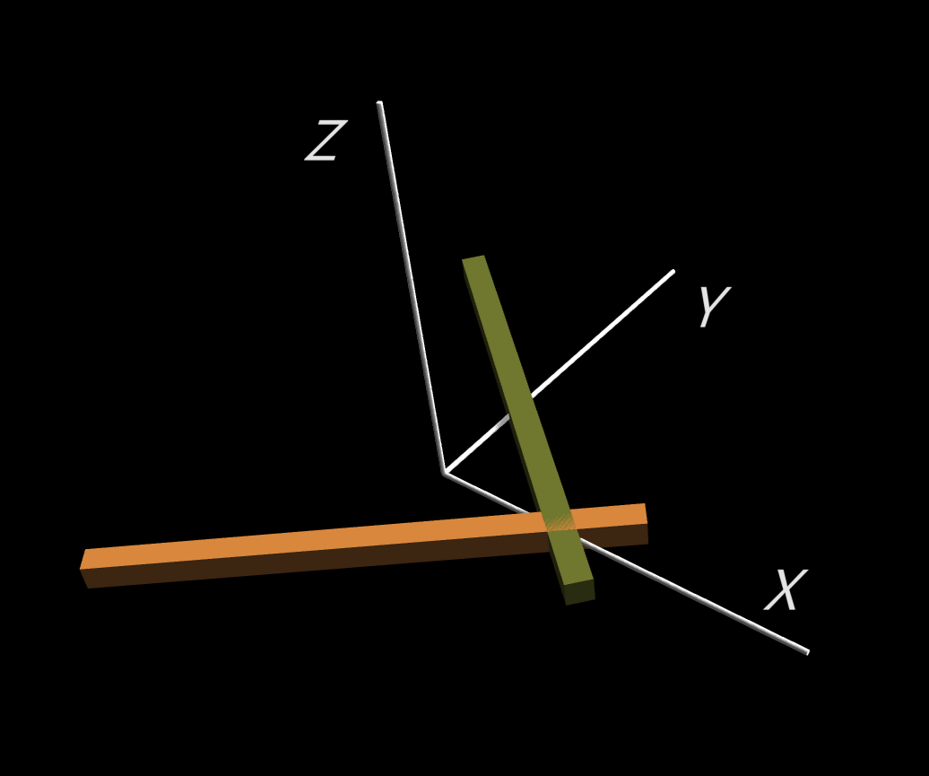

Body fixed coordinate system B with the axises $XYZ$

In each coordinate system, the inertia ellipsoid and the invariable plane are represented by the following expressions.

Inertia Ellipsoid : \[ I_X X^2 + I_Y Y^2 + I_Z Z^2 = 1, \]
where $I_X$, $I_Y$, and $I_Z$ are the inertia moment around the principal axis $X$, $Y$, and $Z$, respectively.

Invariable Plane ; \[ \vec r\cdot\vec L = \sqrt{2 K}; \qquad \vec r := (x, y, z), \quad \mbox{with $K$ being the rotation kinetic energy.} \]

Equations used in the simulation

Equations of motion : Euler equation is the equation of motion represented by the angular velocity vector $\vec\omega$ in the body fixed coordinate system with the principal axises of inertia. Without external force, the angular momentum vector $\vec L$ is constant \[ {d\vec L\over dt} = \left({\partial\vec L\over\partial t}\right)_B + \vec\omega\times\vec L = 0, \] where \[ \left({\partial\vec L\over\partial t}\right)_B := {d L_X\over dt}\hat e_X + {d L_Y\over dt}\hat e_Y + {d L_Z\over dt}\hat e_Z \] represents apparent rate of time change of $\vec L$ in System B. Thus, Euler equation is given by \begin{equation} \left\{\begin{array}{rl}\displaystyle {d\omega_X\over dt} &\displaystyle ={I_Y-I_Z\over I_X}\,\omega_Y\,\omega_Z, \\ \displaystyle {d\omega_Y\over dt} &\displaystyle ={I_Z-I_X\over I_Y}\,\omega_Z\,\omega_X, \\ \displaystyle {d\omega_Z\over dt} &\displaystyle ={I_X-I_Y\over I_Z}\,\omega_X\,\omega_Y. \end{array}\right. \end{equation} This is a set of non-linear equations, therefore its solution cannot be expressed by a superposition of normal modes.

Quaternion representation of rotation : Euler equation is given in the body fixed coordinate system B, thus the solution should be converted into the laboratory system S in order to see the motion from the laboratory.

There are two methods to express the coordinate transformation of rotational between System B and System S: one that uses Euler angles and the other that uses Quaternion. Although Euler angle method is easier to understand intuitively, there exists a singular point in the transformation between Euler angles and the angular velocities, and the numerical integration fails near the singularity. Therefore, it is preferable to use the quaternion method for numerics.

Suppose the vector $\vec a=(a_x, a_y, a_z)$ is transformed to the vector $\vec b=(b_x, b_y, b_z)$ by the rotaion of the angle $\theta$ around the axis $\hat n$. Then the rotation is represented by the quaternion $R_q$ as \[ b_q = R_q\, a_q R_q^{-1}; \qquad R_q = \exp\left[ {\theta\over 2}\,\hat n_q\right] = \cos{\theta\over 2} + \hat n_q \sin{\theta\over 2}, \] where $\hat n$ is a unit vector and \[ a_q := a_x \hat i + a_y \hat j + a_z \hat k, \quad b_q := b_x \hat i + b_y \hat j + b_z \hat k, \quad n_q := n_x \hat i + n_y \hat j + n_z \hat k. \] Here, we have introduced the basis elements of quaternion, $\hat i$, $\hat j$, and $\hat k $, which satisfy \[ \hat i^2 = \hat j^2 =\hat k^2 = \hat i\hat j\hat k =-1 . \]

Transformation from the body fixed system B to the laboratory system S : Consider a vector $\vec a$, which is expressed as \[ \vec a =: a_x \vec e_x + a_y \vec e_y + a_z \vec e_z \] in System S by the basis vectors of the laboratory coordinate $xyz$. Suppose that the same vector $\vec a$ is also expressed as \[ \vec a =: a_X \vec e_X + a_Y \vec e_Y + a_Z \vec e_Z \] in System B by the basis vectors of the body fixed coordinate $XYZ$.

Using these components, let $a^S_q$ and $a^B_q$ be the quaternions defined as \[ a^S_q := a_x \hat i + a_y \hat j + a_z \hat k, \quad a^B_q := a_X \hat i + a_Y \hat j + a_Z \hat k. \] Then, there exists a quaternion $R_q$ which transforms from $a^B_q$ to $a^S_q$ as \begin{equation} a^S_q = R_q a^B_q R_q^{-1}. % \tag{A} \end{equation}

If the angular velocity $\vec\omega$ of System B relative to System S is given, this quaternion $R_q$ can be obtained by solving the equation \begin{equation} {dR_q\over dt} = {1\over 2}\, R_q \omega^B_q, % \tag{B} \end{equation} where $\omega^B_q$ is the quaternion corresponding to the angular velocity $\vec\omega$ of System B in terms of the basis of System B, namely, \[ \vec\omega =: \omega_X \vec e_X + \omega_Y \vec e_Y + \omega_Z \vec e_Z, \qquad \omega^B_q:= \omega_X\hat i + \omega_Y\hat j + \omega_Z\hat k. \] Eq.(B) can be expressed by the components as \begin{equation} {d\over dt} \left(\begin{array}{c} R_W \\ R_X \\ R_Y \\ R_Z \end{array}\right) ={1\over 2} \left(\begin{array}{cccc} 0, & -\omega_X, & -\omega_Y, & -\omega_Z \\ \omega_X, & 0, & \omega_Z, & -\omega_Y \\ \omega_Y, & -\omega_Z, & 0, & \omega_X \\ \omega_Z, & \omega_Y, & -\omega_X, & 0 \end{array}\right) \left(\begin{array}{c} R_W \\ R_X \\ R_Y \\ R_Z \end{array}\right), % \tag{C} \end{equation} where \[ R_q := R_W + R_X \hat i + R_Y\hat j + R_Z\hat k. \]

Eq.(C) may be numerically integrated with Euler equation for $(\omega_X,\omega_Y, \omega_Z)$, thus the orientation of the rigid body can be calculated by $R_q$ using Eq.(A).

Derivation of Eq.(B) :

Let $\vec r$ be the position vector of a point mass that is fixed to the body fixed coordinate B, and suppose that $\vec r=\vec r^0$ at the time $t=0$. If the body fixed coordinate B with the $XYZ$ axises rotates by the angular velocity $\vec\omega$ relative to the laboratory system S with the $xyz$ axises, the velocity of the point mass $\vec v$ is given by \[ \vec v = {d\vec r\over dt} = \vec\omega\times\vec r. \tag{1} \]
On the other hand, let us introduce \[ r^S_q:= x\hat i + y\hat j + z\hat k, \qquad r^0_q:= x^0\hat i + y^0\hat j + z^0\hat k, \] then we have \[ r^S_q = R_q r^0_q R_q^{-1}, \] from which we obtain \begin{eqnarray} v^S_q & := & {dr^S_q\over dt} = {dR_q\over dt}r^0_q R_q^{-1} + R_q r^0_q {d R_q^{-1}\over dt} \\ & = & \Omega_q r^S_q - r^S_q\Omega_q. \tag{2} \end{eqnarray} Here, we have defined \[ \Omega_q:= {dR_q\over dt}R_q^{-1} = - R_q{dR_q^{-1}\over dt}. \tag{3} \]
By comparing Eq.(1) with Eq.(2), we have \[ \Omega_q = {1\over 2}\,\omega_q^S. \] Using this, Eq.(B) is derived from Eq.(3) as \[ {dR_q\over dt} = {1\over 2}\,\omega_q^S R_q = {1\over 2}\, R_q \omega_q^B, \] where we have used \[ \omega_q^S = R_q \omega_q^B R_q^{-1} \] in the last equality. ■