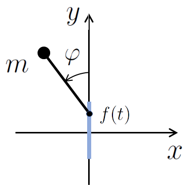
 First, let us consider the case where the vibration is imposed
vertically on the pivot;
\[ f(t) = f\sin(\Omega t) .
\]
First, let us consider the case where the vibration is imposed
vertically on the pivot;
\[ f(t) = f\sin(\Omega t) .
\]
By inserting Eq.(2) into Eq.(1), we may obtain the approximate equation \begin{align*} \ddot\Phi(t) + \textcolor{red}{\ddot\xi(t) } & = \left( \omega_0^2 + {\ddot f(t)\over \ell}\right) \sin\big(\Phi(t)+\xi(t)\big) \\ & \approx \left( \omega_0^2 + \textcolor{red}{{\ddot f(t)\over \ell}}\right) \Big( \sin\Phi(t) + \textcolor{red}{\xi(t)\, \cos\Phi(t)} \Big), \tag{3} \end{align*} where we have used $\Phi\ll\xi$.
Assuming that both $\xi(t)$ and $f(t)$ vibrate by the angular frequency $\Omega$, the magnitudes of the related terms in Eq.(3) may be estimated as \[ \ddot\xi \sim \Omega^2\xi,\quad {\ddot f(t)\over\ell}\sin\Phi \sim \Omega^2{f\over\ell},\quad \omega_0^2\xi\cos\Phi\sim \omega_0^2\xi,\quad {\ddot f(t)\over\ell}\,\xi\cos\Phi \sim \Omega^2{f\over\ell}\,\xi . \] If we adopt $\Omega\gg\omega_0$ and $\xi\sim f/\ell$, then we have the relations among these terms \[ \ddot\xi,\quad {\ddot f(t)\over\ell}\sin\Phi \qquad\gg\qquad \omega_0^2\xi\cos\Phi,\quad {\ddot f(t)\over\ell}\,\xi\cos\Phi. \] The two large terms should balance in Eq.(3) \[ \ddot\xi(t) = {\ddot f(t)\over\ell}\,\sin\Phi(t). \] Noting that $\Phi(r)$ is slowly varying, we can approximate as \[ \xi(t)\approx {f(t)\over\ell}\,\sin\Phi(t). \] After inserting this into Eq.(3) and averaging over the period of vibration $2\pi/\Omega$, we obtain \begin{align*} \ddot\Phi(t) & = \omega_0^2 \sin\Phi(t) + \omega_0^2\,\overline{\xi(t)}\,\cos\Phi(t) + \overline{\ddot f(t) f(t)\over \ell^2}\sin\Phi(t)\cos\Phi(t) \\ & = \omega_0^2 \sin\Phi(t) - {\Omega^2f^2\over 2 \ell^2}\sin\Phi(t)\cos\Phi(t) \\ & := -{d\over d\Phi} U_{\rm eff}(\Phi) . \tag{4} \end{align*} Here, we have used $\overline{\xi(t)}=0$ and $U_{\rm eff}(\Phi)$ is the effective potential for the slow variable $\Phi$: \[ U_{\rm eff}(\Phi):= \omega_0^2\cos\Phi + {\Omega^2 f^2\over 4\,\ell^2}\sin^2\Phi . \tag{5} \] writing down Eq.(4) in the form of harmonic oscillator, we have \[ m\,{d\big(\ell\dot\Phi\big)\over dt} = -{d\over d(\ell\Phi)}\left( mg\ell\cos\Phi + \textcolor{red}{{1\over 2}m \overline{\big(\ell\dot\xi\,\big)^2 }} \right); \qquad \dot\xi(t) := {\Omega f(t)\over\ell}\sin\Phi, \] thus the second term in the effective potential may be considered as the time average of the kinetic energy of the vibration due to external force.
Expanding Eq.(5) by $\Phi$ as \[ U_{\rm eff} (\Phi) = \omega_0^2\left[ 1 +{1\over 2}\left( -1 + {1\over 2}\left({\Omega f\over\omega_0\ell}\right)^2\right)\Phi^2 + O\big(\Phi^4\big)\right], \] thus the inverted state $\Phi=0$ is stabilized when \[ f\,\Omega > \sqrt 2\; \ell\,\omega_0 . \]
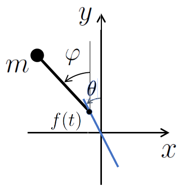 Similar analysis leads us to the effective potential
\[
U_{\rm eff}(\Phi) =
\omega_0^2\cos\Phi
+ {\Omega^2 f^2\over 4\,\ell^2}\sin^2\big(\Phi-\theta\big) .
\]
The term due to the external vibration has the minima
in the directions $\theta$ and $\theta+\pi$.
Similar analysis leads us to the effective potential
\[
U_{\rm eff}(\Phi) =
\omega_0^2\cos\Phi
+ {\Omega^2 f^2\over 4\,\ell^2}\sin^2\big(\Phi-\theta\big) .
\]
The term due to the external vibration has the minima
in the directions $\theta$ and $\theta+\pi$.